42 how to add data labels to a pie chart in excel

Pie Chart in Excel | How to Create Pie Chart - EDUCBA Step 1: Select the data to go to Insert, click on PIE, and select 3-D pie chart. Step 2: Now, it instantly creates the 3-D pie chart for you. Step 3: Right-click on the pie and select Add Data Labels. This will add all the values we are showing on the slices of the pie. Add a DATA LABEL to ONE POINT on a chart in Excel All the data points will be highlighted. Click again on the single point that you want to add a data label to. Right-click and select ' Add data label '. This is the key step! Right-click again on the data point itself (not the label) and select ' Format data label '. You can now configure the label as required — select the content of ...

Display data point labels outside a pie chart in a paginated report ... Create a pie chart and display the data labels. Open the Properties pane. On the design surface, click on the pie itself to display the Category properties in the Properties pane. Expand the CustomAttributes node. A list of attributes for the pie chart is displayed. Set the PieLabelStyle property to Outside. Set the PieLineColor property to Black.

How to add data labels to a pie chart in excel

Add or remove data labels in a chart - support.microsoft.com Click the data series or chart. To label one data point, after clicking the series, click that data point. In the upper right corner, next to the chart, click Add Chart Element > Data Labels. To change the location, click the arrow, and choose an option. If you want to show your data label inside a text bubble shape, click Data Callout. c# - Add data labels to excel pie chart - Stack Overflow I am drawing a pie chart with some data: private void DrawFractionChart(Excel.Worksheet activeSheet, Excel.ChartObjects xlCharts, Excel.Range xRange, Excel.Range yRange) { Excel.ChartObject ... Add data labels to excel pie chart. Ask Question Asked 9 years, 9 months ago. Modified 5 years, 10 months ago. Viewed 9k times Add data labels and callouts to charts in Excel 365 - EasyTweaks.com The steps that I will share in this guide apply to Excel 2021 / 2019 / 2016. Step #1: After generating the chart in Excel, right-click anywhere within the chart and select Add labels . Note that you can also select the very handy option of Adding data Callouts.

How to add data labels to a pie chart in excel. How to Create Pie Charts in Excel (In Easy Steps) Select the pie chart. 9. Click the + button on the right side of the chart and click the check box next to Data Labels. 10. Click the paintbrush icon on the right side of the chart and change the color scheme of the pie chart. Result: 11. Right click the pie chart and click Format Data Labels. 12. How to Make a Pie Chart in Excel - WinBuzzer Select your data and press the pie icon in the "Insert" tab of the ribbon. You can then choose which type of pie chart you want. In our case, that's the basic "2-D Pie" option. However ... How to Customize Your Excel Pivot Chart Data Labels - dummies To add data labels, just select the command that corresponds to the location you want. To remove the labels, select the None command. If you want to specify what Excel should use for the data label, choose the More Data Labels Options command from the Data Labels menu. Excel displays the Format Data Labels pane. How to Create and Format a Pie Chart in Excel - Lifewire To add data labels to a pie chart: Select the plot area of the pie chart. Right-click the chart. Select Add Data Labels . Select Add Data Labels. In this example, the sales for each cookie is added to the slices of the pie chart. Change Colors

Pie of Pie Chart in Excel - Inserting, Customizing, Formatting Inserting a Pie of Pie Chart. Let us say we have the sales of different items of a bakery. Below is the data:-. To insert a Pie of Pie chart:-. Select the data range A1:B7. Enter in the Insert Tab. Select the Pie button, in the charts group. Select Pie of Pie chart in the 2D chart section. Inserting Data Label in the Color Legend of a pie chart Small and Medium Business. Public Sector. Internet of Things (IoT) Azure Partner Community. Expand your Azure partner-to-partner network. Microsoft Tech Talks. Bringing IT Pros together through In-Person & Virtual events. MVP Award Program. Find out more about the Microsoft MVP Award Program. Adding Data Labels to Your Chart (Microsoft Excel) To add data labels, follow these steps: Activate the chart by clicking on it, if necessary. Choose Chart Options from the Chart menu. Excel displays the Chart Options dialog box. Make sure the Data Labels tab is selected. (See Figure 1.) The left side of the dialog box shows the different types of data labels you can choose. (The available ... Microsoft Excel Tutorials: Add Data Labels to a Pie Chart To add the numbers from our E column (the viewing figures), left click on the pie chart itself to select it: The chart is selected when you can see all those blue circles surrounding it. Now right click the chart. You should get the following menu: From the menu, select Add Data Labels. New data labels will then appear on your chart:

How to add data labels from different column in an Excel chart? Right click the data series in the chart, and select Add Data Labels > Add Data Labels from the context menu to add data labels. 2. Click any data label to select all data labels, and then click the specified data label to select it only in the chart. 3. Change the format of data labels in a chart To get there, after adding your data labels, select the data label to format, and then click Chart Elements > Data Labels > More Options. To go to the appropriate area, click one of the four icons ( Fill & Line, Effects, Size & Properties ( Layout & Properties in Outlook or Word), or Label Options) shown here. How to insert data labels to a Pie chart in Excel 2013 - YouTube This video will show you the simple steps to insert Data Labels in a pie chart in Microsoft® Excel 2013. Content in this video is provided on an "as is" basi... Possible to add second data label to pie chart? - Excel Help Forum Re: Possible to add second data label to pie chart? Create the composite label in a worksheet column by concatenating the data in other cells and the nextline character, CHR (10). Now, use this composite label column as the source for Rob Bovey's add-in. -- Regards, Tushar Mehta Excel, PowerPoint, and VBA add-ins, tutorials

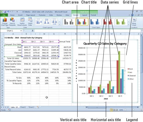
Getting to Know the Parts of an Excel 2010 Chart - dummies

How to Make a Pie Chart in Excel: 10 Steps (with Pictures) 1. Open Microsoft Excel. It resembles a white "E" on a green background. If you would rather make a chart from data you already have, double-click the Excel document that contains the data to open it and proceed to the next section. 2. Click Blank workbook (PC) or Excel Workbook (Mac).

Breaking down hierarchical data with Treemap and Sunburst charts - Microsoft 365 Blog

How to add or move data labels in Excel chart? - ExtendOffice In Excel 2013 or 2016. 1. Click the chart to show the Chart Elements button . 2. Then click the Chart Elements, and check Data Labels, then you can click the arrow to choose an option about the data labels in the sub menu. See screenshot: In Excel 2010 or 2007. 1. click on the chart to show the Layout tab in the Chart Tools group. See ...

Share :