39 excel chart labels from cells
Excel charts: add title, customize chart axis, legend and data labels Select the chart and go to the Chart Tools tabs ( Design and Format) on the Excel ribbon. Right-click the chart element you would like to customize, and choose the corresponding item from the context menu. Use the chart customization buttons that appear in the top right corner of your Excel graph when you click on it. How to Print Labels from Excel - Lifewire To label legends in Excel, select a blank area of the chart. In the upper-right, select the Plus ( +) > check the Legend checkbox. Then, select the cell containing the legend and enter a new name. How do I label a series in Excel? To label a series in Excel, right-click the chart with data series > Select Data.
Apply Custom Data Labels to Charted Points - Peltier Tech Select an individual label (two single clicks as shown above, so the label is selected but the cursor is not in the label text), type an equals sign in the formula bar, click on the cell containing the label you want, and press Enter. The formula bar shows the link (=Sheet1!$D$3). Repeat for each of the labels.

Excel chart labels from cells
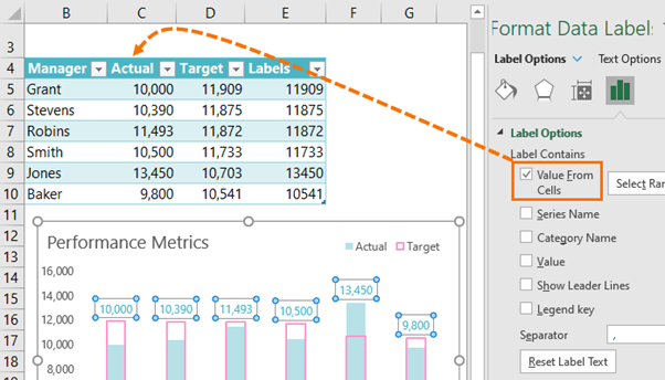
How to Customize Your Excel Pivot Chart Data Labels The Data Labels command on the Design tab's Add Chart Element menu in Excel allows you to label data markers with values from your pivot table. When you click the command button, Excel displays a menu with commands corresponding to locations for the data labels: None, Center, Left, Right, Above, and Below. Using the CONCAT function to create custom data labels for an Excel chart Use the chart skittle (the "+" sign to the right of the chart) to select Data Labels and select More Options to display the Data Labels task pane. Check the Value From Cells checkbox and select the cells containing the custom labels, cells C5 to C16 in this example. It is important to select the entire range because the label can move based ... How to add data labels from different column in an Excel chart? This method will guide you to manually add a data label from a cell of different column at a time in an Excel chart. 1. Right click the data series in the chart, and select Add Data Labels > Add Data Labels from the context menu to add data labels. 2.
Excel chart labels from cells. Excel: Add labels to data points in XY chart - Stack Overflow Excel 2013 introduced the capability to label a chart series with data from cells, after many years of users begging for it. Select the series, and add data labels. Select the data labels and format them. Under Label Options in the task pane, look for Label Contains, select the Value From Cells option, and select the range containing the label ... Chart Labels & Cell References - Excel Charting & Graphing - Board ... then on your chart select the label and instead of typing direct into the box click on the formula bar at the top of the page and then type a reference to the cell containing the earlier formula eg. Your label should now contain "Profits for Year 1999" (assuming of course that cell A1 contained the value "1999") Thank you very much. excel - Using VBA to create charts with data labels based on cell ... With x-axis data labels being set to the top row of headings (the blue range) With series labels being set according to the three group labels immediately to the left of the data. (the orange range) So far, all I've succeeded doing is the first one, based on this answer, resulting in the following code: Excel Charts - Option "Label contains value From cells" disappear 2016. Platform. Windows. Mar 11, 2021. #5. Lasa1 said: Original file is .xls and the new book is .xlsx. Thanks, indeed that was the root casue. I saved the original file with .xlsx, close and reopen and nowthe lable option " value from cells" is available.Thanks.
How to Use Cell Values for Excel Chart Labels - How-To Geek Select the chart, choose the "Chart Elements" option, click the "Data Labels" arrow, and then "More Options." Uncheck the "Value" box and check the "Value From Cells" box. Select cells C2:C6 to use for the data label range and then click the "OK" button. The values from these cells are now used for the chart data labels. Excel Data Labels - Value from Cells To automatically update titles or data labels with changes that you make on the worksheet, you must reestablish the link between the titles or data labels and the corresponding worksheet cells. For data labels, you can reestablish a link one data series at a time, or for all data series at the same time. Create Waffle Chart in Excel - Quick Guide - Excelkid The positive side is that the waffle chart is open to changes because it is connected to cell number N7. In other words, any changes in cell N7 will lead to a new state of the whole chart. At this point, further attempts will be made to introduce related labels to the KPI value in cell N7. #2 - Create Chart Labels Link a chart title, label, or text box to a worksheet cell On the Format tab, in the Current Selection group, click the arrow next to the Chart Elements box, and then click the chart element that you want to use. In the formula bar, type an equal sign ( = ). In the worksheet, select the cell that contains the data that you want to display in the title, label, or text box on the chart.
Excel tutorial: How to customize axis labels Here you'll see the horizontal axis labels listed on the right. Click the edit button to access the label range. It's not obvious, but you can type arbitrary labels separated with commas in this field. So I can just enter A through F. When I click OK, the chart is updated. So that's how you can use completely custom labels. Creating a chart with dynamic labels - Microsoft Excel 365 1. Right-click on the chart and in the popup menu, select Add Data Labels and again Add Data Labels : 2. Do one of the following: Right-click on any data label and select Format Data Labels... in the popup menu: On the Format Data Labels pane, on the Label Options section, in the Label Contains group, check the Value From Cells option and then ... How to Add Data Labels to an Excel 2010 Chart - dummies On the Chart Tools Layout tab, click Data Labels→More Data Label Options. The Format Data Labels dialog box appears. You can use the options on the Label Options, Number, Fill, Border Color, Border Styles, Shadow, Glow and Soft Edges, 3-D Format, and Alignment tabs to customize the appearance and position of the data labels. How to Add Labels to Scatterplot Points in Excel - Statology Next, click anywhere on the chart until a green plus (+) sign appears in the top right corner. Then click Data Labels, then click More Options… In the Format Data Labels window that appears on the right of the screen, uncheck the box next to Y Value and check the box next to Value From Cells.
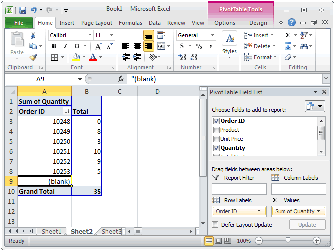
MS Excel 2010: Hide Blanks in a Pivot Table
Add or remove data labels in a chart - Microsoft Support Click Label Options and under Label Contains, pick the options you want. Use cell values as data labels You can use cell values as data labels for your chart. Right-click the data series or data label to display more data for, and then click Format Data Labels. Click Label Options and under Label Contains, select the Values From Cells checkbox.

35 Label Cells In Excel - Label Design Ideas 2020
How to Add Axis Labels in Excel Charts - Step-by-Step (2022) - Spreadsheeto How to add axis titles 1. Left-click the Excel chart. 2. Click the plus button in the upper right corner of the chart. 3. Click Axis Titles to put a checkmark in the axis title checkbox. This will display axis titles. 4. Click the added axis title text box to write your axis label.
Excel for Business Statistics
Automatically set chart axis labels from cell contents The (tick) labels occur at each > major tick along the axis. > > You can link the text of an axis title to a particular cell. Select the > axis title, press the equals key, and select the cell. > > This also works with the chart title, individual data labels, and text > boxes. > > - Jon > ------- > Jon Peltier, Microsoft Excel MVP
35 Excel Cell Label - Labels Information List
Chart.ApplyDataLabels method (Excel) | Microsoft Docs The type of data label to apply. True to show the legend key next to the point. The default value is False. True if the object automatically generates appropriate text based on content. For the Chart and Series objects, True if the series has leader lines. Pass a Boolean value to enable or disable the series name for the data label.

Ablebits.com Ultimate Suite for Excel - 60+ professional tools to get more power from your Excel
Creating a chart with dynamic labels - Microsoft Excel 2016 1. Right-click on the chart and in the popup menu, select Add Data Labels and again Add Data Labels : 2. Do one of the following: For all labels: on the Format Data Labels pane, in the Label Options, in the Label Contains group, check Value From Cells and then choose cells: For the specific label: double-click on the label value, in the popup ...

Automatically hide labels in line chart if cell is blank - Excel - Stack Overflow
How to add or move data labels in Excel chart? - ExtendOffice In Excel 2013 or 2016. 1. Click the chart to show the Chart Elements button . 2. Then click the Chart Elements, and check Data Labels, then you can click the arrow to choose an option about the data labels in the sub menu. See screenshot: In Excel 2010 or 2007. 1. click on the chart to show the Layout tab in the Chart Tools group. See ...
Custom Excel Chart Label Positions • My Online Training Hub
Data Label in Charts Excel 2007 - Microsoft Community I saw in the new 2013 version of Excel there is an option to create a custom data range in Format Chart Data Labels called "Value From Cells" I do not see this as an option in Excel 2007. is there a way to include a custom range for Chart Data Labels in 2007? This thread is locked. You can follow the question or vote as helpful, but you cannot ...

Chart in Excel Cells - YouTube
Dynamically Label Excel Chart Series Lines - My Online Training Hub Step 1: Duplicate the Series. The first trick here is that we have 2 series for each region; one for the line and one for the label, as you can see in the table below: Select columns B:J and insert a line chart (do not include column A). To modify the axis so the Year and Month labels are nested; right-click the chart > Select Data > Edit the ...

Excel: How to make an Excel-lent bull's-eye chart
How to Change Excel Chart Data Labels to Custom Values? - Chandoo.org You can change data labels and point them to different cells using this little trick. First add data labels to the chart (Layout Ribbon > Data Labels) Define the new data label values in a bunch of cells, like this: Now, click on any data label. This will select "all" data labels. Now click once again.
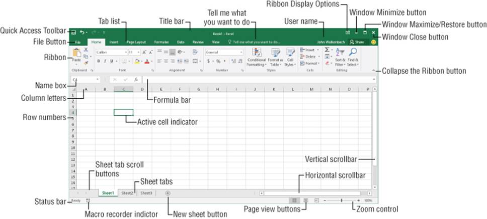
Screenshot of the Excel screen with labeled parts.
Create Dynamic Chart Data Labels with Slicers - Excel Campus Typically a chart will display data labels based on the underlying source data for the chart. In Excel 2013 a new feature called "Value from Cells" was introduced. This feature allows us to specify the a range that we want to use for the labels. Since our data labels will change between a currency ($) and percentage (%) formats, we need a ...
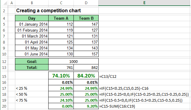
Creating a funny competition chart
How to add data labels from different column in an Excel chart? This method will guide you to manually add a data label from a cell of different column at a time in an Excel chart. 1. Right click the data series in the chart, and select Add Data Labels > Add Data Labels from the context menu to add data labels. 2.
35 Label Cells In Excel - Label Design Ideas 2020
Using the CONCAT function to create custom data labels for an Excel chart Use the chart skittle (the "+" sign to the right of the chart) to select Data Labels and select More Options to display the Data Labels task pane. Check the Value From Cells checkbox and select the cells containing the custom labels, cells C5 to C16 in this example. It is important to select the entire range because the label can move based ...

Fill All Blank Cells in an Excel Range With a Desired Value | EXCEL UNPLUGGED
How to Customize Your Excel Pivot Chart Data Labels The Data Labels command on the Design tab's Add Chart Element menu in Excel allows you to label data markers with values from your pivot table. When you click the command button, Excel displays a menu with commands corresponding to locations for the data labels: None, Center, Left, Right, Above, and Below.
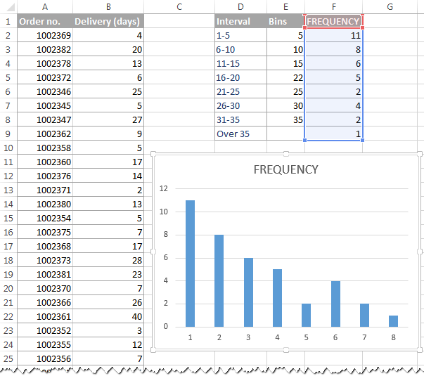
How to make a histogram in Excel 2019, 2016, 2013 and 2010

How to Create and Interpret a Correlation Matrix in Excel - Statology

Excel compare list
Post a Comment for "39 excel chart labels from cells"