38 excel graph data labels
chandoo.org › wp › change-data-labels-in-chartsHow to Change Excel Chart Data Labels to Custom Values? May 05, 2010 · Now, click on any data label. This will select “all” data labels. Now click once again. At this point excel will select only one data label. Go to Formula bar, press = and point to the cell where the data label for that chart data point is defined. Repeat the process for all other data labels, one after another. See the screencast. Adding rich data labels to charts in Excel 2013 - Microsoft 365 Blog The data labels up to this point have used numbers and text for emphasis. Putting a data label into a shape can add another type of visual emphasis. To add a data label in a shape, select the data point of interest, then right-click it to pull up the context menu. Click Add Data Label, then click Add Data Callout .
Excel Chart Data Labels - Microsoft Community Right-click a data point on your chart, from the context menu choose Format Data Labels ..., choose Label Options > Label Contains Value from Cells > Select Range. In the Data Label Range dialog box, verify that the range includes all 26 cells. When I paste your data into a worksheet, the XY Scatter data is in A2:B27, and the data labels are in ...

Excel graph data labels
Edit titles or data labels in a chart - support.microsoft.com The first click selects the data labels for the whole data series, and the second click selects the individual data label. Right-click the data label, and then click Format Data Label or Format Data Labels. Click Label Options if it's not selected, and then select the Reset Label Text check box. Top of Page How to add data labels from different column in an Excel chart? Right click the data series in the chart, and select Add Data Labels > Add Data Labels from the context menu to add data labels. 2. Click any data label to select all data labels, and then click the specified data label to select it only in the chart. 3. How to Place Labels Directly Through Your Line Graph in Microsoft Excel Right-click on top of one of those circular data points. You'll see a pop-up window. Click on Add Data Labels. Your unformatted labels will appear to the right of each data point: Click just once on any of those data labels. You'll see little squares around each data point. Then, right-click on any of those data labels.
Excel graph data labels. › linking-a-graph-inLinking a graph in PowerPoint to the Excel data so the graph ... Each method starts with you creating the graph in Excel first, because we will be copying the graph created in Excel into the PowerPoint slide. Method 1: Basic Paste. After you have created the graph in Excel, click on it and copy it (press Ctrl+C or click the copy button on the Home ribbon). Switch to your PowerPoint slide. How to create a chart (graph) in Excel and save it as template 22.10.2015 · 3. Inset the chart in Excel worksheet. To add the graph on the current sheet, go to the Insert tab > Charts group, and click on a chart type you would like to create.. In Excel 2013 and Excel 2016, you can click the Recommended Charts button to view a gallery of pre-configured graphs that best match the selected data.. In this example, we are creating a 3-D … Add a DATA LABEL to ONE POINT on a chart in Excel Steps shown in the video above: Click on the chart line to add the data point to. All the data points will be highlighted. Click again on the single point that you want to add a data label to. Right-click and select ' Add data label ' This is the key step! Right-click again on the data point itself (not the label) and select ' Format data label '. How to I rotate data labels on a column chart so that they are ... To change the text direction, first of all, please double click on the data label and make sure the data are selected (with a box surrounded like following image). Then on your right panel, the Format Data Labels panel should be opened. Go to Text Options > Text Box > Text direction > Rotate
Excel tutorial: How to use data labels Generally, the easiest way to show data labels to use the chart elements menu. When you check the box, you'll see data labels appear in the chart. If you have more than one data series, you can select a series first, then turn on data labels for that series only. You can even select a single bar, and show just one data label. How to hide zero data labels in chart in Excel? - ExtendOffice Sometimes, you may add data labels in chart for making the data value more clearly and directly in Excel. But in some cases, there are zero data labels in the chart, and you may want to hide these zero data labels. Here I will tell you a quick way to hide the zero data labels in Excel at once. Hide zero data labels in chart Excel charts: add title, customize chart axis, legend and data labels ... Click anywhere within your Excel chart, then click the Chart Elements button and check the Axis Titles box. If you want to display the title only for one axis, either horizontal or vertical, click the arrow next to Axis Titles and clear one of the boxes: Click the axis title box on the chart, and type the text. Excel.ChartDataLabels class - Office Add-ins | Microsoft Docs The request context associated with the object. This connects the add-in's process to the Office host application's process. Specifies the format of chart data labels, which includes fill and font formatting. Specifies the horizontal alignment for chart data label. See Excel.ChartTextHorizontalAlignment for details.
How to format axis labels as thousands/millions in Excel? Reuse Anything: Add the most used or complex formulas, charts and anything else to your favorites, and quickly reuse them in the future. More than 20 text features: Extract Number from Text String; Extract or Remove Part of Texts; Convert Numbers and Currencies to English Words. Merge Tools: Multiple Workbooks and Sheets into One; Merge Multiple Cells/Rows/Columns Without Losing Data; Merge ... How to Make a Bar Graph in Excel: 9 Steps (with Pictures) 02.05.2022 · It's easy to spruce up data in Excel and make it easier to interpret by converting it to a bar graph. A bar graph is not only quick to see and understand, but it's also more engaging than a list of numbers. This wikiHow article will teach you how to make a bar graph of your data in Microsoft Excel. How To Use Dynamic Data Labels To Create Interactive Excel Charts To create a column chart with dynamic data labels, you need to follow these given steps. Select the data & Create a Combo Chart. Now select the column chart for revenue data and a line chart with marker for data labels Add Data Labels to the Line Chart With Marker. After then remove the Line Color and Marker Color. Move data labels - support.microsoft.com Right-click the selection > Chart Elements > Data Labels arrow, and select the placement option you want. Different options are available for different chart types. For example, you can place data labels outside of the data points in a pie chart but not in a column chart.
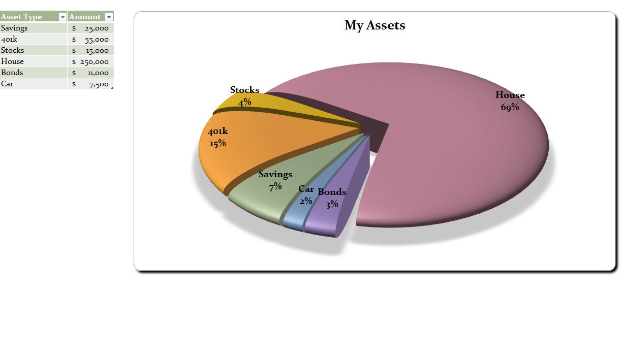
Excel Pie Chart | Pie Chart Excel
Change the format of data labels in a chart To get there, after adding your data labels, select the data label to format, and then click Chart Elements > Data Labels > More Options. To go to the appropriate area, click one of the four icons ( Fill & Line, Effects, Size & Properties ( Layout & Properties in Outlook or Word), or Label Options) shown here.
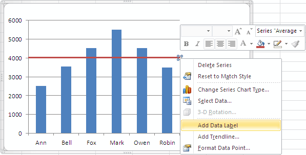
How To Add an Average Line to Column Chart in Excel 2010 - Excel How To
› Make-a-Bar-Graph-in-ExcelHow to Make a Bar Graph in Excel: 9 Steps (with Pictures) May 02, 2022 · Customize your graph's appearance. Once you decide on a graph format, you can use the "Design" section near the top of the Excel window to select a different template, change the colors used, or change the graph type entirely.
Regression Analysis - Confidence Interval of the Line of Best Fit
Add / Move Data Labels in Charts - Excel & Google Sheets Adding Data Labels Click on the graph Select + Sign in the top right of the graph Check Data Labels Change Position of Data Labels Click on the arrow next to Data Labels to change the position of where the labels are in relation to the bar chart Final Graph with Data Labels

E-xcel Tuts: Add Data Labels to Excel Charts
How to Change Excel Chart Data Labels to Custom Values? 05.05.2010 · Now, click on any data label. This will select “all” data labels. Now click once again. At this point excel will select only one data label. Go to Formula bar, press = and point to the cell where the data label for that chart data point is defined. Repeat the process for all other data labels, one after another. See the screencast.

Create a Line Chart in Excel - Easy Excel Tutorial
› excel › how-to-add-total-dataHow to Add Total Data Labels to the Excel Stacked Bar Chart Apr 03, 2013 · Step 4: Right click your new line chart and select “Add Data Labels” Step 5: Right click your new data labels and format them so that their label position is “Above”; also make the labels bold and increase the font size. Step 6: Right click the line, select “Format Data Series”; in the Line Color menu, select “No line”
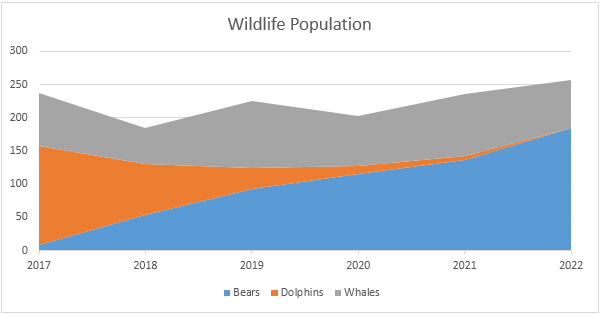
Area Chart in Excel - Easy Excel Tutorial
Excel Chart Data Labels-Modifying Orientation - Microsoft Community In reply to PaulaAB's post on September 13, 2016. Hi Paula, You can right click on the data label part then select Format Axis. Click on the Size & Properties tab then adjust the Text Direction or Custom Angle. Thanks,
34 Label Data Points In Excel - Best Labels Ideas 2020
How to add or move data labels in Excel chart? - ExtendOffice In Excel 2013 or 2016. 1. Click the chart to show the Chart Elements button . 2. Then click the Chart Elements, and check Data Labels, then you can click the arrow to choose an option about the data labels in the sub menu. See screenshot: In Excel 2010 or 2007. 1. click on the chart to show the Layout tab in the Chart Tools group. See ...
Post a Comment for "38 excel graph data labels"